hepi.plot

Submodules

• hepi.plot.plot

Attributes

map_vplot
scatter_vplot
fig
axs
lines
labels

Classes

Input

Input for computation and scans.

Functions

get_output_dir()	Get the output directory.
replace_macros(s)
get_name(pid)	Get the latex name of a particle.
title(i[, axe, scenario, diff_L_R, extra, cms_energy, ...])	Sets the title on axis axe.
energy_plot(dict_list, y[, yscale, xaxis, yaxis, label])	Plot energy on the x-axis.
combined_mass_plot(dict_list, y, part[, label])
combined_plot(dict_list, x, y[, label])
mass_plot(dict_list, y, part[, logy, yaxis, yscale, ...])
mass_vplot(dict_list, y, part[, logy, yaxis, yscale, ...])
get_mass(l, iid)	Get the mass of particle with id iid out of the list in the "slha" element in the dict.
plot(dict_list, x, y[, label, xaxis, yaxis, ratio, K, ...])	Creates a plot based on the entries x`and `y in dict_list.
index_open(var, idx)
slha_data(li, index_list)
slha_plot(li, x, y, **kwargs)
vplot(x, y[, label, xaxis, yaxis, logy, yscale, ...])	Creates a plot based on the values in x`and `y.
mass_mapplot(dict_list, part1, part2, z[, logz, ...])
mapplot(dict_list, x, y, z[, xaxis, yaxis, zaxis])	Examples
scatterplot(dict_list, x, y, z[, xaxis, yaxis, zaxis])	Scatter map 2d.
err_plt(axes, x, y[, label, error])
scale_plot(dict_list, vl[, seven_point_band, cont, ...])	Creates a scale variance plot with 5 panels (xline).
central_scale_plot(dict_list, vl[, cont, error, ...])	Creates a scale variance plot with 3 panels (ystacked).
init_double_plot([figsize, sharex, sharey, gridspec_kw])	Initialze subplot for Ratio/K plots with another figure below.

Package Contents

class hepi.plot.Input(order, energy, particle1, particle2, slha, pdf_lo, pdf_nlo, mu_f=1.0, mu_r=1.0, pdfset_lo=0, pdfset_nlo=0, precision=0.001, max_iters=50, invariant_mass='auto', result='total', pt='auto', id='', model='', update=True)

Bases: hepi.util.DictData

Input for computation and scans.

Variables:

• order (Order) – LO, NLO or NLO+NLL computation.

• energy (int) – CMS energy in GeV.

• energyhalf (int) – Halfed energy.

• particle1 (int) – PDG identifier of the first final state particle.

• particle2 (int) – PDG identifier of the second final state particle.

• slha (str) – File path of for the base slha. Modified slha files will be used if a scan requires a change of the input.

• pdf_lo (str) – LO PDF name.

• pdf_nlo (str) – NLO PDF name.

• pdfset_lo (int) – LO PDF member/set id.

• pdfset_nlo (int) – NLO PDF member/set id.

• pdf_lo_id (int) – LO PDF first member/set id.

• pdf_nlo_id (int) – NLO PDF first member/set id.

• mu (double) – central scale factor.

• mu_f (double) – Factorization scale factor.

• mu_r (double) – Renormalization scale factor.

• precision (double) – Desired numerical relative precision.

• max_iters (int) – Upper limit on integration iterations.

• invariant_mass (str) – Invariant mass mode ‘auto = sqrt((p1+p2)^2)’ else value.

• pt (str) – Transverse Momentum mode ‘auto’ or value.

• result (str) – Result type ‘total’/’pt’/’ptj’/’m’.

• id (str) – Set an id of this run.

• model (str) – Path for MadGraph model.

• update (bool) – Update dependent mu else set to zero.

Parameters:

• order (hepi.order.Order)

• energy (float)

• particle1 (int)

• particle2 (int)

• slha (str)

• pdf_lo (str)

• pdf_nlo (str)

order

energy

energyhalf

particle1

particle2

slha

pdf_lo

pdfset_lo = 0

pdf_nlo

pdfset_nlo = 0

pdf_lo_id = 0

pdf_nlo_id = 0

mu_f = 1.0

mu_r = 1.0

precision = 0.001

max_iters = 50

invariant_mass = 'auto'

pt = 'auto'

result = 'total'

id = ''

model = ''

mu = 0.0

has_gluino()

Return type:

bool

has_neutralino()

Return type:

bool

has_charginos()

Return type:

bool

has_weakino()

Return type:

bool

has_squark()

Return type:

bool

has_slepton()

Return type:

bool

hepi.plot.get_output_dir()

Get the output directory.

Returns:

out_dir

Return type:

str

hepi.plot.replace_macros(s)

Parameters:

s (str)

Return type:

str

hepi.plot.get_name(pid)

Get the latex name of a particle.

Parameters:

pid (int) – PDG Monte Carlo identifier for the particle.

Returns:

Latex name.

Return type:

str

Examples

>>> get_name(21)
'g'
>>> get_name(1000022)
'\\tilde{\\chi}_{1}^{0}'

hepi.plot.title(i, axe=None, scenario=None, diff_L_R=None, extra='', cms_energy=True, pdf_info=True, id=False, **kwargs)

Sets the title on axis axe.

Parameters:

i (hepi.input.Input)

hepi.plot.energy_plot(dict_list, y, yscale=1.0, xaxis='E [GeV]', yaxis='$\\sigma$ [pb]', label=None, **kwargs)

Plot energy on the x-axis.

hepi.plot.combined_mass_plot(dict_list, y, part, label=None, **kwargs)

hepi.plot.combined_plot(dict_list, x, y, label=None, **kwargs)

hepi.plot.mass_plot(dict_list, y, part, logy=True, yaxis='$\\sigma$ [pb]', yscale=1.0, label=None, xaxis=None, **kwargs)

hepi.plot.mass_vplot(dict_list, y, part, logy=True, yaxis='$\\sigma$ [pb]', yscale=1.0, label=None, mask=None, **kwargs)

hepi.plot.get_mass(l, iid)

Get the mass of particle with id iid out of the list in the “slha” element in the dict.

Returns

list of float : masses of particles in each element of the dict list.

Parameters:

• l (dict)

• iid (int)

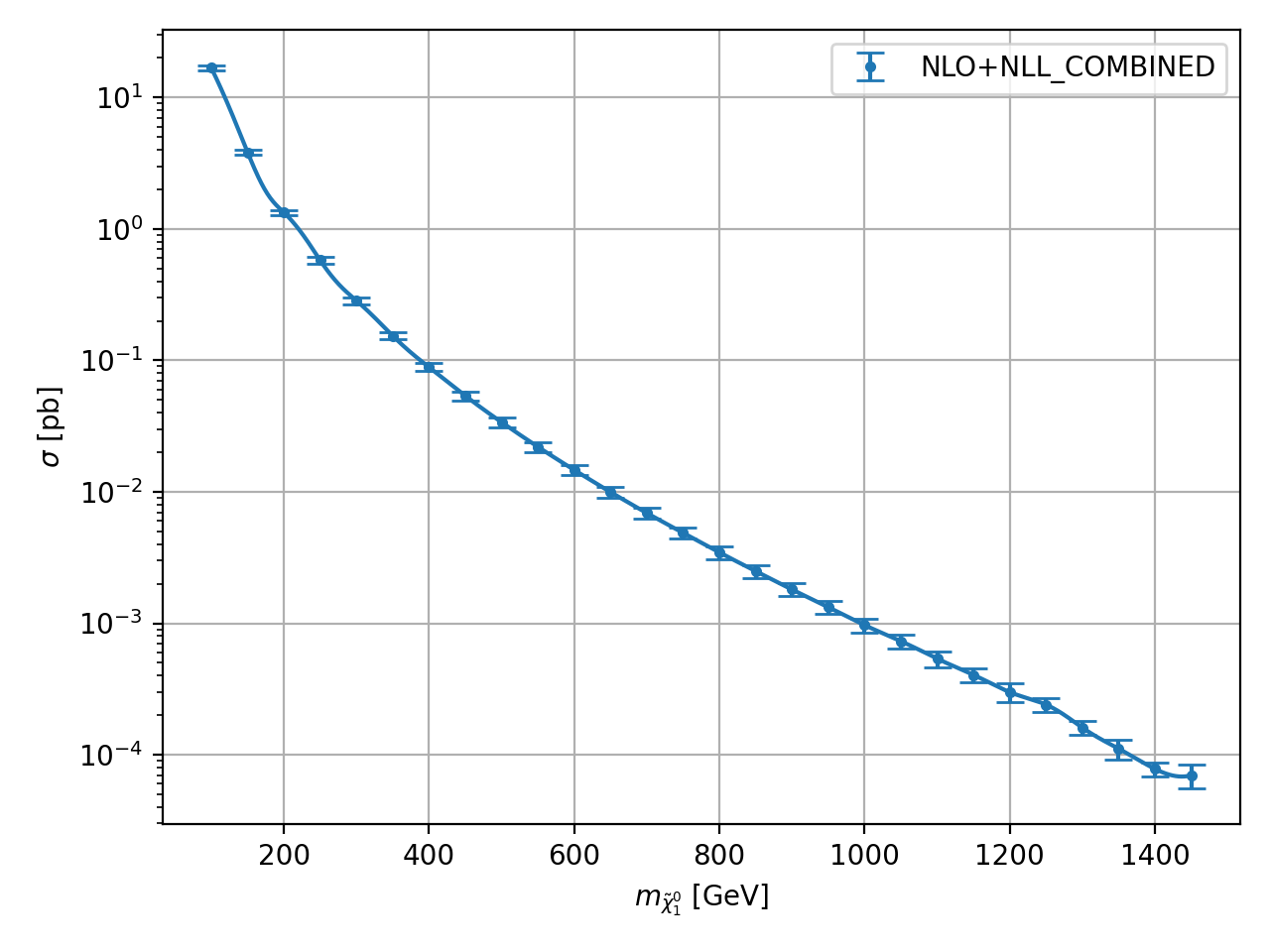
hepi.plot.plot(dict_list, x, y, label=None, xaxis='M [GeV]', yaxis='$\\sigma$ [pb]', ratio=False, K=False, K_plus_1=False, logy=True, yscale=1.0, mask=None, **kwargs)

Creates a plot based on the entries x`and `y in dict_list.

Examples

>>> import urllib.request
>>> import hepi
>>> dl = hepi.load(urllib.request.urlopen(
... "https://raw.githubusercontent.com/fuenfundachtzig/xsec/master/json/pp13_hino_NLO%2BNLL.json"
... ))
>>> hepi.plot(dl,"N1","NLO_PLUS_NLL_COMBINED",xaxis="$m_{\\tilde{\\chi}_1^0}$ [GeV]")

(Source code, png, hires.png, pdf)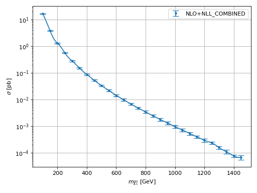

Return type:

None

hepi.plot.index_open(var, idx)

hepi.plot.slha_data(li, index_list)

hepi.plot.slha_plot(li, x, y, **kwargs)

hepi.plot.vplot(x, y, label=None, xaxis='E [GeV]', yaxis='$\\sigma$ [pb]', logy=True, yscale=1.0, interpolate=True, plot_data=True, data_color=None, mask=-1, fill=False, data_fmt='.', fmt='-', print_area=False, sort=True, **kwargs)

Creates a plot based on the values in x`and `y.

hepi.plot.mass_mapplot(dict_list, part1, part2, z, logz=True, zaxis='$\\sigma$ [pb]', zscale=1.0, label=None)

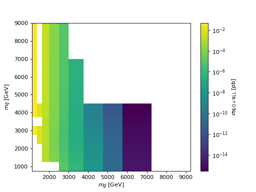
hepi.plot.mapplot(dict_list, x, y, z, xaxis=None, yaxis=None, zaxis=None, **kwargs)

Examples

>>> import urllib.request
>>> import hepi

>>> dl = hepi.load(urllib.request.urlopen(
... "https://raw.githubusercontent.com/APN-Pucky/xsec/master/json/pp13_SGmodel_GGxsec_NLO%2BNLL.json"
... ),dimensions=2)
>>> hepi.mapplot(dl,"gl","sq","NLO_PLUS_NLL_COMBINED",xaxis="$m_{\\tilde{g}}$ [GeV]",yaxis="$m_{\\tilde{q}}$ [GeV]" , zaxis="$\\sigma_{\\mathrm{NLO+NLL}}$ [pb]")

(Source code, png, hires.png, pdf)

hepi.plot.map_vplot

hepi.plot.scatter_vplot

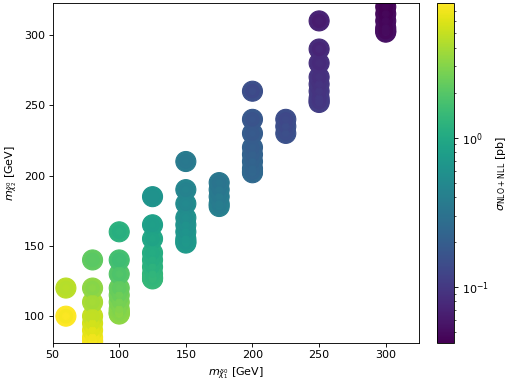
hepi.plot.scatterplot(dict_list, x, y, z, xaxis=None, yaxis=None, zaxis=None, **kwargs)

Scatter map 2d. Central color is the central value, while the inner and outer ring are lower and upper bounds of the uncertainty interval.

Examples

>>> import urllib.request
>>> import hepi
>>> dl = hepi.load(urllib.request.urlopen(
... "https://raw.githubusercontent.com/APN-Pucky/xsec/master/json/pp13_hinosplit_N2N1_NLO%2BNLL.json"
... ),dimensions=2)
>>> hepi.scatterplot(dl,"N1","N2","NLO_PLUS_NLL_COMBINED",xaxis="$m_{\\tilde{\\chi}_1^0}$ [GeV]",yaxis="$m_{\\tilde{\\chi}_2^0}$ [GeV]" , zaxis="$\\sigma_{\\mathrm{NLO+NLL}}$ [pb]")

(Source code, png, hires.png, pdf)

hepi.plot.fig = None

hepi.plot.axs = None

hepi.plot.lines = []

hepi.plot.labels = []

hepi.plot.err_plt(axes, x, y, label=None, error=False)

hepi.plot.scale_plot(dict_list, vl, seven_point_band=False, cont=False, error=True, li=None, plehn_color=False, yscale=1.0, unit='pb', yaxis=None, **kwargs)

Creates a scale variance plot with 5 panels (xline).

hepi.plot.central_scale_plot(dict_list, vl, cont=False, error=True, yscale=1.0, unit='pb', yaxis=None)

Creates a scale variance plot with 3 panels (ystacked).

hepi.plot.init_double_plot(figsize=(6, 8), sharex=True, sharey=False, gridspec_kw={'height_ratios': [3, 1]})

Initialze subplot for Ratio/K plots with another figure below.