Function Plot

[1]:

from smpl import plot
import numpy as np
import smpl
import math
smpl.__version__

[1]:

'1.3.0'

without uncertainties

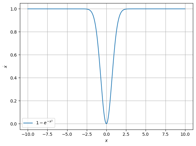
\(\dot x = 1- \exp(- x^2)\)

Fixed point \(x = 0\) and

\(\ddot x = -2x \exp(-x^2) \implies \ddot x(x = 0)=0\)

only metastable for \(x\lt0\)

[2]:

plot.function( lambda x : 1- np.exp(-x**2), xaxis="$x$", yaxis="$\\dot x$",xmin=-10, xmax=10 )

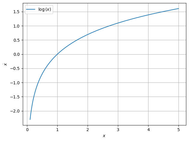
../../../_images/example_plot_functions_funcs_4_0.png

\(\dot x = \ln x\)

Fixed point \(x = 1\)

\[\ddot x = \frac{1}{x} \implies \ddot x(x=1) = 1 > 0\]

\(\implies\) unstable

[3]:

plot.function( lambda x : np.log(x), xaxis="$x$", yaxis="$\\dot x$",xmin=0.1, xmax=5 )

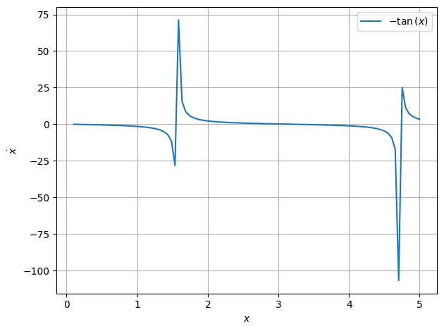
../../../_images/example_plot_functions_funcs_6_0.png

\(\dot x = -\tan x\)

Fixed points for \(x=0\) or \(x=\pm n\pi\) with \(n\in \mathbb{N}\)

\[\ddot x = -\frac{1}{\cos^2(x)}\]

\[\ddot x(x=0) = -1 \lt 0\]

\[\ddot x(x=n \pi) = -1 \lt 0\]

\(\implies\) stable

[4]:

plot.function( lambda x : -np.tan(x), xaxis="$x$", yaxis="$\\dot x$",xmin=0.1, xmax=5,steps=100 )

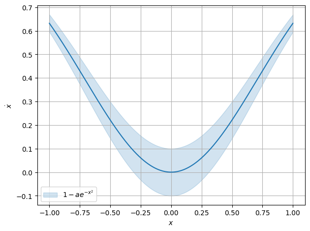
../../../_images/example_plot_functions_funcs_8_0.png

with uncertainties

[5]:

import uncertainties as unc
a = unc.ufloat(1,0.1)

[6]:

plot.function(lambda x : 1- a*np.exp(-x**2), xaxis="$x$", yaxis="$\\dot x$",xmin=-1, xmax=1,sigmas=1 )

../../../_images/example_plot_functions_funcs_11_0.png

Complex

[7]:

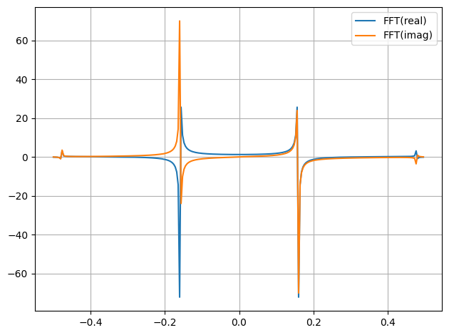
from smpl.stat import fft
y = np.sin(np.arange(256))
print(len(fft(y)))
plot.data(*fft(y),label="FFT",fmt="-")

/__w/smpl/smpl/smpl/plot.py:852: UserWarning: The figure layout has changed to tight
  plt.tight_layout()

[7]:

(None, None)

../../../_images/example_plot_functions_funcs_13_3.png

[8]:

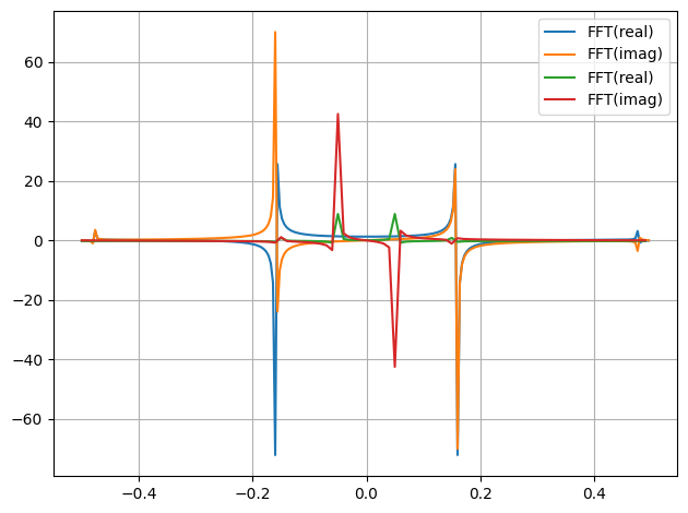
from smpl.stat import fft
plot.data(*fft(np.sin(np.arange(256))),*fft(np.sin(1/np.pi*np.arange(100))),label="FFT",fmt="-")

[8]:

[(None, None), (None, None)]

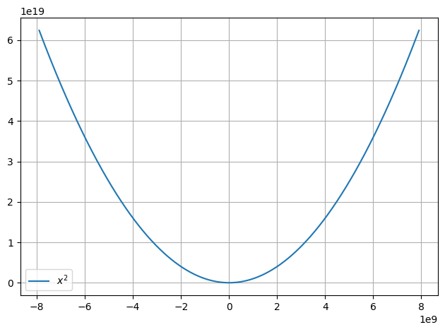
../../../_images/example_plot_functions_funcs_14_1.png

without xmin and xmax

xmin and xmax will have to be guessed

[9]:

from smpl import plot
plot.function(lambda x: x**2,)

../../../_images/example_plot_functions_funcs_16_0.png

[10]:

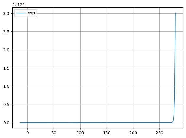
from smpl import plot
import numpy as np
def f(x):
    return np.exp(x)
plot.function(f,label="exp")

/tmp/ipykernel_1773/1264896925.py:4: RuntimeWarning: overflow encountered in exp
  return np.exp(x)

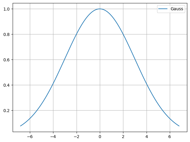
../../../_images/example_plot_functions_funcs_17_1.png

[11]:

from smpl import plot
from smpl import functions as f
def gauss(x):
    """Gauss"""
    return f.gauss(x,0,1,3,0)
plot.function(gauss)

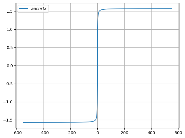
../../../_images/example_plot_functions_funcs_18_0.png

[12]:

def gauss(x):
    return np.arctan(x)
plot.function(gauss)

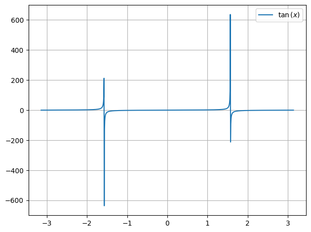
../../../_images/example_plot_functions_funcs_19_0.png

[13]:

def gauss(x):
    return np.tan(x)
plot.function(gauss)

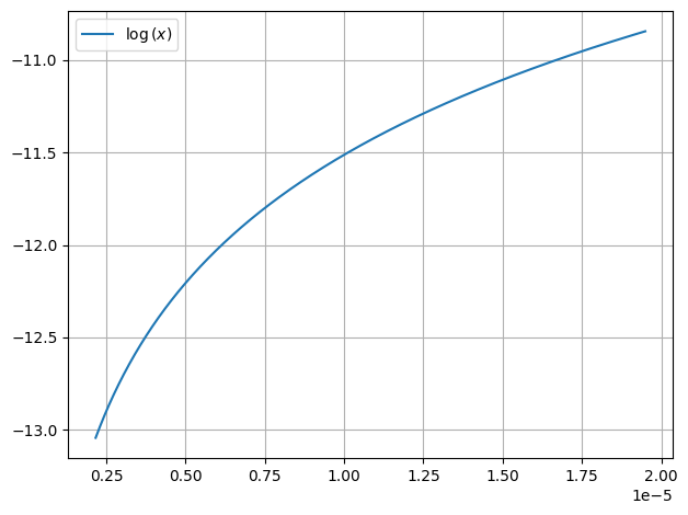
../../../_images/example_plot_functions_funcs_20_0.png

[14]:

def gauss(x):
    return np.log(x)
plot.function(gauss)

/tmp/ipykernel_1773/455222689.py:2: RuntimeWarning: invalid value encountered in log
  return np.log(x)

../../../_images/example_plot_functions_funcs_21_1.png

[15]:

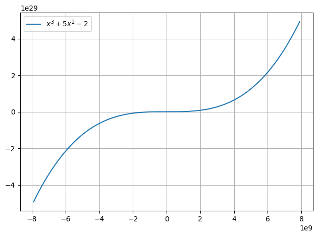
def gauss(x):
    return x**3+5*x**2-2
plot.function(gauss)

../../../_images/example_plot_functions_funcs_22_0.png

[16]:

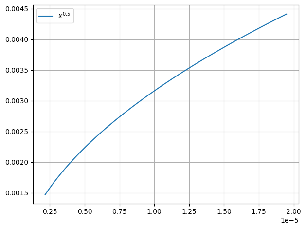
def gauss(x):
    return x**0.5
plot.function(gauss)

/tmp/ipykernel_1773/1404190211.py:2: RuntimeWarning: invalid value encountered in sqrt
  return x**0.5

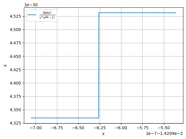
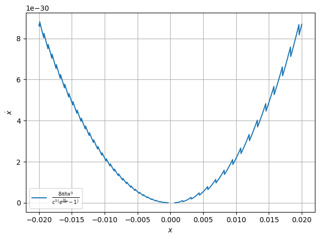
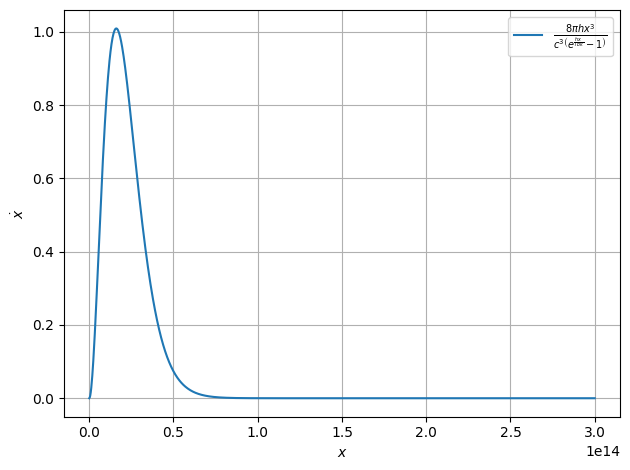
../../../_images/example_plot_functions_funcs_23_1.png

Guessing the interesting regions of a function can’t always be correct/satisfactory, especially in numerical unstable regions:

[17]:

c=299792458#m/s
h=4.13566769692*10**-15#eVs
kb=8.617333262*10**-5#eV/K
T=273
def Strahlungsgesetz(x):
    return 8*np.pi/c**3*h*x**3/(np.exp((h*x)/(kb*T))-1)
plot.function(Strahlungsgesetz,xaxis="$x$", yaxis="$\\dot x$")

/tmp/ipykernel_1773/4149904953.py:6: RuntimeWarning: overflow encountered in exp
  return 8*np.pi/c**3*h*x**3/(np.exp((h*x)/(kb*T))-1)
/tmp/ipykernel_1773/4149904953.py:6: RuntimeWarning: invalid value encountered in divide
  return 8*np.pi/c**3*h*x**3/(np.exp((h*x)/(kb*T))-1)
/tmp/ipykernel_1773/4149904953.py:6: RuntimeWarning: divide by zero encountered in divide
  return 8*np.pi/c**3*h*x**3/(np.exp((h*x)/(kb*T))-1)
/github/home/.cache/pypoetry/virtualenvs/smpl-4sWS420u-py3.8/lib/python3.8/site-packages/scipy/optimize/_optimize.py:790: RuntimeWarning: invalid value encountered in subtract
  np.max(np.abs(fsim[0] - fsim[1:])) <= fatol):
/github/home/.cache/pypoetry/virtualenvs/smpl-4sWS420u-py3.8/lib/python3.8/site-packages/scipy/misc/_common.py:144: RuntimeWarning: invalid value encountered in multiply
  val += weights[k]*func(x0+(k-ho)*dx,*args)

../../../_images/example_plot_functions_funcs_25_1.png

[18]:

plot.function(Strahlungsgesetz,xaxis="$x$", yaxis="$\\dot x$",xmin=1e-7-2e-2,xmax=1e-7+2e-2)

/tmp/ipykernel_1773/4149904953.py:6: RuntimeWarning: divide by zero encountered in divide
  return 8*np.pi/c**3*h*x**3/(np.exp((h*x)/(kb*T))-1)

../../../_images/example_plot_functions_funcs_26_1.png

[19]:

plot.function(Strahlungsgesetz,xaxis="$x$", yaxis="$\\dot x$",xmin=1,xmax=0.3e15)

../../../_images/example_plot_functions_funcs_27_0.png

[ ]: